After a request to add more axes to the previous simple variable fonts tutorial the follow up escalated a bit. Since there are several files I thought it might be better to put them on github.
Best posts made by jo
-
More variable fonts nonsenseposted in Code snippets

-
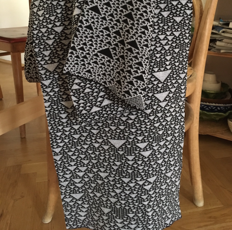
Rotating rectangles based on an artpiece by Vera Molnarposted in Tutorials
Intro
This is based on an art work by Vera Molnar (a pioneer in the field of generative art).
This script will generate a pattern with randomly rotated rectangles – using two nested loops.Code and explanation
Lets start with the default settings of DrawBot:
fill color is black, a white background and a canvas with a width and height of 1000 units.First we define how many rows and columns we want to have in the drawing and assign this value to the variable amount
amount = 24Next we want to define the size of each cell in the grid. We want to calculate this value and not define a fixed value so it updates automatically. To calculate the width of the cell we call the width() function which returns the width of the canvas (in our case the default value of 1000). We divide this value by the amount of cells (stored in the variable amount). Since we want to have a margin around the drawing we just add 2 to the amount.
cell_s = width() / (amount + 2)Since we want the squares rotated by 45 degrees to touch at the corners we need to calculate the size of the rectangles.
With a rotation of 45 degrees this can be done quite easily by dividing the cell size by the square root of 2.rect_s = cell_s / sqrt(2)Now we should have all the numbers ready to start drawing the pattern. To apply the margin we first shift the origin of the drawing one cell size to the right and to the top. We do this by calling the translate() function with the parameters of one cell size in the x direction and the y direction
translate(cell_s, cell_s)Now lets start to loop in the x direction as many times as defined in the amount variable
for x in range(amount):And then for each x value do the same in the y direction. So our total amount of cells will be the square of the amount (24 * 24 = 576 cells).
for y in range(amount):Before we call the rotate() function lets first shift the origin with the translate() function. Since we want to revert back to the default state (with no rotation) after we have drawn a rectangle let’s call the savedState() function first:
with savedState():Now let’s do the shifting: Shift x times the cell size to the left and y times the cell size to the top. Since we want the rotation to be happening in the center of the cell we need to add half a cell size in each direction.
translate( x * cell_s + cell_s/2, y * cell_s + cell_s/2 )We only want to do the rotation on some of the cells. So we just call the random() function which returns a randomly generated value between 0 and 1. If this value is higher than 0.5 (which on average should be in half of the cases) let’s do the rotation:
            if random() > .5:
            	rotate(45)
Finally lets draw a rectangle by calling the rect() function. The rectangle should be drawn half a cell size to the left and bottom to compensate for the extra translation from before:
rect(-rect_s/2, -rect_s/2, rect_s, rect_s)To save the image lets call the saveImage() function and give a path and file name:
saveImage('~/Desktop/Vera_Molnar_rotating_rects.png')Everything put together
amount = 24
cell_s = width() / (amount + 2)

rect_s = cell_s / sqrt(2)
translate( cell_s, cell_s)

for x in range(amount):
    for y in range(amount):
        with savedState():
            translate( x * cell_s + cell_s/2, y * cell_s + cell_s/2 )
            if random() > .5:
            	rotate(45)
            rect(-rect_s/2, -rect_s/2, rect_s, rect_s)

# saveImage('~/Desktop/Vera_Molnar_rotating_rects.png')
Image

-
Vera Molnar re-codedposted in Code snippets
Vera Molnar is a great computer generated arts pioneer and is still working. I could not resist to emulate and try to recode some of her artworks. Using drawbot to do so is great fun and pretty easy — one can only wonder about the struggles she had to overcome. With all due respect here is a link to github with my humble attempts.
-
Animated Müller-Lyer illusionposted in Code snippets
nautil.us has a nice blogpost of optical illusions. I could not resist the attempt to build one of them in drawbot.
pw = ph = 400 # define variables to set width and height of the canvas
cols = 14 # define how many columns there should be
rows = 4 # define how many rows there should be
pages = 30 # define how many frames the gif should have. more pages mean slower movement

angle_diff = 2 * pi/pages # we want the loop to make one full circle. 2 times pi is 360 degrees. Divided by the amount of pages this gives us the angle difference between pages.

gap = pw/(cols+1) # calculate the gap between the lines.
l   = (ph - 2 * gap)/rows # calculate the length of the line.

for p in range(pages):
    newPage(pw, ph)
    translate(gap, gap)
    fill(None)
    strokeWidth(2)
    for x in range(cols):
        y_off = cos( 3 * pi * x/cols + angle_diff * p ) * gap/2 # calculate how high or low the arrowhead should be
        for y in range(rows+1):
            stroke(1,0 ,0) if y % 2 == 0 else stroke(0, 0, 1)
            if y < rows:
                line((x*gap, y*l), (x*gap, y*l+l))
            stroke(0)
            y_off *= -1 # switch to change direction
            line( (x*gap, y*l), (x*gap - gap/2, y*l - y_off) )
            line( (x*gap, y*l), (x*gap + gap/2, y*l - y_off) )

# saveImage('~/Desktop/opti_illu.gif')
this should generate something like this:
-
RE: Cellular automatonposted in Code snippets
the script could be used to get a scarf knitted.
good idea. thanks for the tipp @frederikrule 122 on one side which makes the other side rule 161
-
RE: How to mirror/flip a object?posted in General Discussion
the mirrored drawing is probably happening outside your canvas. keep in mind that every transformation (scale, skew, rotation, etc) is always starting from the origin. so a mirroring from the default origin (left, bottom corner) will be to the left or below your canvas. see the example below with a shifted origin.
pw = 1000
ph = 400
txt = "SHADE"
newPage(pw, ph)
translate(0, 160) # shift the origin up a bit
fontSize(300)
text(txt, (pw/2, 0), align = 'center')
scale(x=1, y=-.5) # the mirroring
text(txt, (pw/2, 0), align = 'center')
-
RE: A deeper bevel on lineJoin()?posted in General Discussion
@mauricemeilleur I don’t know how Crouwel defined his rules. but to me the corner-rule seems like an integral part of the design.
I had a look at my code and tried to tidy the worst bits. some of the angle calculations seem very inefficient but ¯\(ツ)/¯ here it is:
EDIT 2018-05-28 changed the code to simplify some of the horrible trigonometry and there now is the
sq_capbool to have squared linecaps.# Draw a 'folded outline' between a set of points. # TO DO: There should be an error message when two dots are closer to each other and the weight. # There should be a warning if the folding is further than the next points. # There should be a warning for collinear points. import math # Just a bunch of points p01 = (894, 334) p02 = (808, 86) p03 = (274, 792) p04 = (481, 920) p05 = (583, 730) p06 = (85, 430) p07 = (318, 100) p08 = (870, 600) p09 = (720, 690) points = [p01, p02, p03, p04, p05, p06, p07, p08, p09] def get_dist(p1, p2): return sqrt( (p2[0] - p1[0] )**2 + (p2[1] - p1[1])**2 ) def calc_angle(p1, p2): return atan2((p2[1] - p1[1]), (p2[0] - p1[0])) def calc_delta(p1, p2, p3): ''' Returns the angle between three points. ''' return calc_angle(p2, p3) - calc_angle(p2, p1) def calc_offset(weight, p1, p2, p3): ''' Returns the x and y "offset" to be added to the points of the polygon. ''' halfWeight = weight/2 if p1 == p2: alpha = calc_angle(p1, p3) b = -sin(alpha) * halfWeight a = cos(alpha) * halfWeight elif p2 == p3: alpha = calc_angle(p1, p3) b = sin(alpha) * halfWeight a = -cos(alpha) * halfWeight else: alpha = calc_angle(p2, p3) delta = calc_delta(p1, p2, p3) xx = halfWeight / sin((delta - pi) / 2) delta_f = (2 * alpha - pi - delta ) / 2 a, b = xx * sin(delta_f), xx * cos(delta_f) return a, b def wrap_line(p1, p2, p3, p4, weight): ''' This draws a polygon around a line. Four points (x,y) and a weight parameter are required. The polygon will be drawn around the two middle points. The first and last points define the angles. ''' a, b = calc_offset(weight, p1, p2, p3) # extend first point x1b, y1b = p2[0] - b, p2[1] - a x1c, y1c = p2[0] + b, p2[1] + a # extend second point c, d = calc_offset(weight, p2, p3, p4) x2b, y2b = p3[0] - d, p3[1] - c x2c, y2c = p3[0] + d, p3[1] + c polygon((x1b, y1b), (x1c, y1c), (x2b, y2b), (x2c, y2c)) # -------------------------------------------------------------------- # The actual drawing fill(0, .4) weight = 180 sq_cap = True if len(points) == 1: rect(points[0][0] - weight/2, points[0][1] - weight/2, weight, weight) for i, point in enumerate(points[:-1]): # print (get_dist(point, points[i+1])) if len(points) == 2: wrap_line(points[i], points[i], points[i+1], points[i+1], weight) else: if i == 0: aaa = calc_angle(points[i], points[i+1]) if sq_cap: point = point[0] - weight/2 * cos(aaa), point[1] - weight/2 * sin(aaa) wrap_line(point, point, points[i+1], points[i+2], weight) elif i == len(points)-2: next_p = points[i+1] aaa = calc_angle(points[i], next_p) if sq_cap: next_p = next_p[0] + weight/2 * cos(aaa), next_p[1] + weight/2 * sin(aaa) wrap_line(points[i-1], points[i], next_p, next_p, weight) else: # print ( calc_delta(points[i-1], points[i], points[i+1]) ) wrap_line(points[i-1], points[i], points[i+1], points[i+2], weight)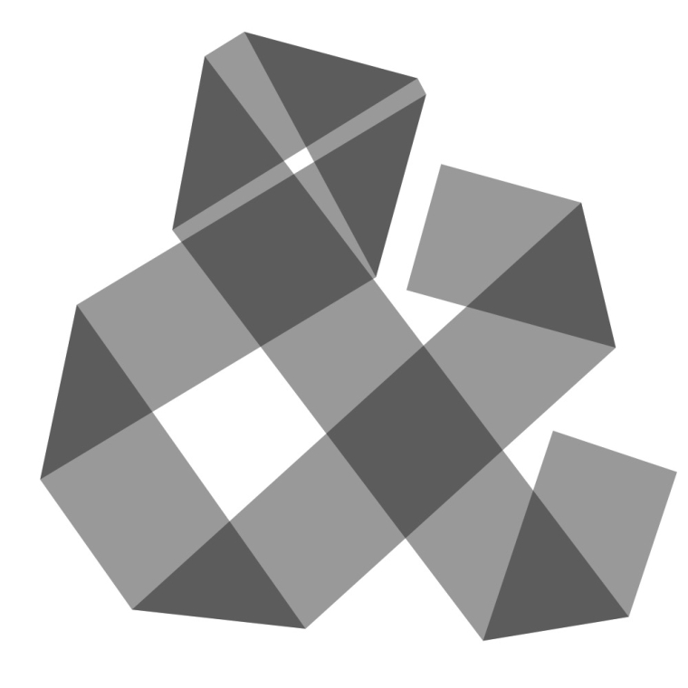
-
RE: Tutorial request: how to animate a variable fontposted in Tutorials
hi there
I will try to give you a basic start with a very simple linear interpolation.–––
Let’s animate some variable fonts.
we are on mac os so lets first see if there are any variable fonts installed on the system
To do this lets iterate through all installed fonts and ask if they do have any font variation axes. the function
listFontVariations()will return this information as anOrderedDictif you supply a font name. Let’s print the name of the font if it returns any variable axes. And then let’s iterate through this information (short code and information on the values that could be set) for every axis and print this as well.for fontName in installedFonts(): variations = listFontVariations(fontName) if variations: print(fontName) for axis_name, dimensions in variations.items(): print (axis_name, dimensions) print ()Depending on your os version you should get a few fonts.
Let’s assume one of the fonts is 'Skia-Regular' and it did print the following information:Skia-Regular wght {'name': 'Weight', 'minValue': 0.4799, 'maxValue': 3.1999, 'defaultValue': 1.0} wdth {'name': 'Width', 'minValue': 0.6199, 'maxValue': 1.2999, 'defaultValue': 1.0}This information can now be used to set some typographic parameters. Let’s use the weight axis (wght) and animate from the minimum to the maximum. To do so we assign these two values to variables.
min_val = listFontVariations('Skia-Regular')['wght']['minValue'] max_val = listFontVariations('Skia-Regular')['wght']['maxValue']Let’s also assign the amount of steps for the interpolation to a variable and the text we want to render.
steps = 10 txt = 'var fonts are fun'The last variable we are going to need is a calculation of the stepsize.
So let’s get the range by subtracting the minimum from the maximum and divide this value by the amount of steps minus one step.step_size = (max_val - min_val) / (steps-1)We should now be ready to loop through the amount of steps.
For every step we make a new page and set the font and font size. We calculate the value for the respective step by multiplying the step_size by the step and add it to the minimum value. The result of this calculation is then used in thefontVariations()function to set the variable font values.for i in range(steps): newPage(1100, 200) font("Skia-Regular") fontSize(120) curr_value = min_val + i * step_size fontVariations(wght= curr_value ) text(txt, (70, 70))Everything put together
for fontName in installedFonts(): variations = listFontVariations(fontName) if variations: print(fontName) for axis_name, dimensions in variations.items(): print (axis_name, dimensions) print () min_val = listFontVariations('Skia-Regular')['wght']['minValue'] max_val = listFontVariations('Skia-Regular')['wght']['maxValue'] steps = 10 txt = 'var fonts are fun' step_size = (max_val - min_val) / (steps-1) for i in range(steps): newPage(1100, 200) font("Skia-Regular") fontSize(120) curr_value = min_val + i * step_size fontVariations(wght= curr_value ) text(txt, (70, 70)) fontSize(20) fontVariations(wght= 1 ) text('Weight axis: %f' % curr_value, (10, 10)) saveImage('~/Desktop/var_fonts_interpol.gif')Final gif
With 20 interpolation steps and with a smaller canvas size.
Any questions or corrections please let me know!
-
Lissajous tableposted in Code snippets
Here is some code to draw a Lissajous table.
Change thefunc_xand/orfunc_y(sin or cos) and/or add some value to thedeltato get other curves.
Well, actually the curves are just polygons.# ---------------------- # lissajous table # ---------------------- # settings cols = 12 rows = 8 cell_s = 80 r_factor = .8 # fraction of the cell size to have a gap between them func_x = cos # should be `sin` or `cos` func_y = sin # should be `sin` or `cos` delta = 0 #pi/3 # some angle in radians density = 360 # amount of points per cell – higher values make nicer curve approximations # ---------------------- # calculated settings radius = (cell_s * r_factor) / 2 step = (2 * pi) / density pw = cell_s * (cols + 1) ph = cell_s * (rows + 1) x_coords = { (col, d) : func_x(step * (col + 1) * d + pi/2 + delta) * radius for col in range(cols) for d in range(density) } y_coords = { (row, d) : func_y(step * (row + 1) * d + pi/2) * radius for row in range(rows) for d in range(density) } # ---------------------- # function(s) def draw_cell(pos, col, row): cx, cy = pos points = [(cx + x_coords[(col, f)], cy + y_coords[(row, f)]) for f in range(density)] polygon(*points) # ---------------------- # drawings newPage(pw, ph) rect(0, 0, pw, ph) fontSize(12) translate(0, ph) fill(1) text('δ\n{0:.2f}°'.format(degrees(delta)), (cell_s * (1 - r_factor)/2, -20)) for col in range(1, cols+1): cx = col * cell_s + cell_s * (1 - r_factor)/2 text('{0}\n{1}'.format(func_x.__name__, col), (cx, -20)) for row in range(1, rows + 1): cy = row * cell_s + cell_s * (1 - r_factor) text('{0}\n{1}'.format(func_y.__name__, row), (cell_s * (1 - r_factor)/2, -cy)) fill(None) stroke(.5) strokeWidth(1) for col in range(cols): for row in range(rows): draw_cell((cell_s * col + cell_s * 1.5, - cell_s * row -cell_s * 1.5), col, row)
-
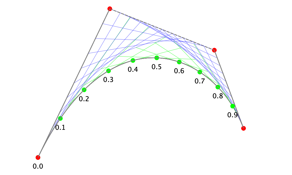
Drawing a circle with Beziersposted in Code snippets
You cannot draw a circle with Beziers.
When I first read this some time ago I was a bit confused.
Why is this not a circle. It sure looks like one.After learning a bit more about curve descriptions and calculations I kind of agree but the quote should better say:
You cannot draw a perfect circle with Beziers.
Getting the best tangent values.
We have a formula to calculate points on a Bezier Curve.
x = (1-t)**3*p1[0] + 3*(1-t)**2*t*t1[0] + 3*(1-t)*t**2*t2[0] + t**3*p2[0]
y = (1-t)**3*p1[1] + 3*(1-t)**2*t*t1[1] + 3*(1-t)*t**2*t2[1] + t**3*p2[1]
p1 and p2 are the two endpoints and t1 and t2 the two tangent points. t is the factor (0-1) at which we want the point on the curve.
On a bezier curve with the following coördinates:
p1 = (1, 0)
p2 = (0, 1)
t1 = (1, tangent_val)
t2 = (tangent_val, 1)
we can calculate the tangent_val if we assume that the point at t=0.5 (halfway the curve) is exactly on the circle. Halfway of a quartercircle is 45 degrees so x and y are both at 1/sqrt(2). If we plug these numbers into the formula we can calculate the tangent value:
1/sqrt(2) = (1-.5)**3*1 + 3*(1-.5)**2*.5*1 + 3*(1-.5)*.5**2*tangent_val + .5**3*0
...
tangent_val = 4*(sqrt(2)-1)/3 ≈ 0.5522847493
With this tangent_val we can calculate other points on the bezier curve. Of which we can calculate the angle in respect to the center point at (0, 0). And with this angle we can use sine and cosine to get the point that would be on a circle.
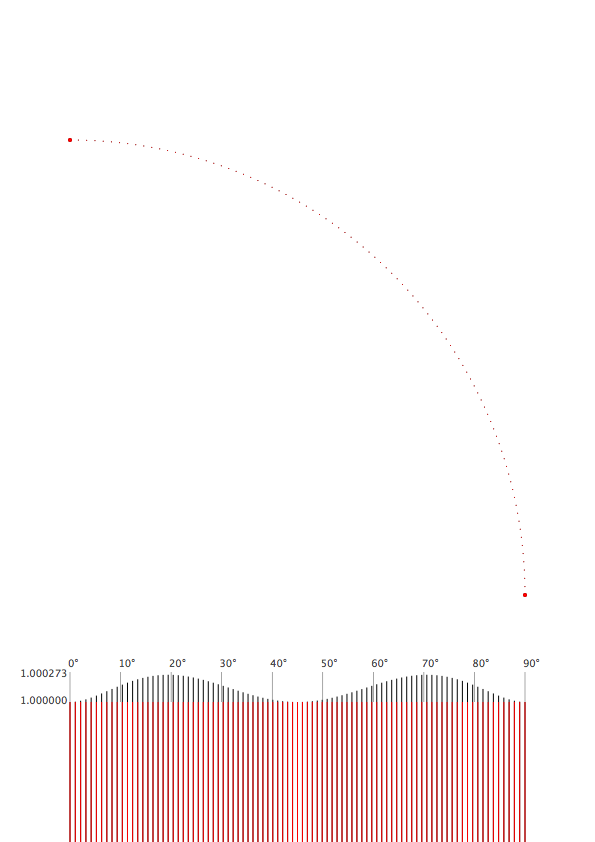
We can also calculate the distance of the bezier point and see where the offset is the biggest. As we can see the difference is really tiny. With a radius of 1 the biggest off value is 1.0002725295591013 (not even one permille). The difference is hardly visible so I added only the top part of a really long bar chart to make it show.
See the image below:
Code
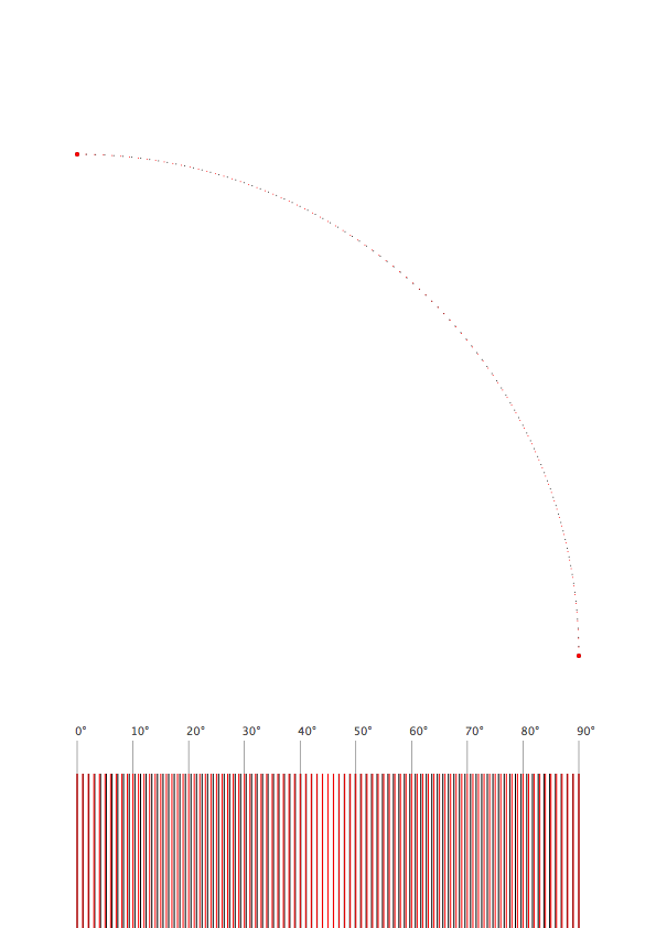
# -------------------
#  settings

pw, ph = 595, 842 #A4
margin = 70

tang = 4*(sqrt(2)-1)/3
r = pw - 2 * margin

density = 90 # amount of points
dia_ = 1 # diameter to draw the points

r_plot = 100000 # this is a magnifying factor to make the tiny difference visible.

r_plot_y = margin - r_plot   #radius plotting
c_plot_y = ph - 3 * margin - r  # circle plotting

# -------------------
#  functions

def get_bezier_p(p1, t1, t2, p2, t):
    ''' get the point on a bezier curve at t (should be between 0 and 1) '''
    x = (1 - t)**3 * p1[0] + 3*(1 - t)**2 * t * t1[0] + 3*(1 - t)* t**2 * t2[0] + t**3 * p2[0]
    y = (1 - t)**3 * p1[1] + 3*(1 - t)**2 * t * t1[1] + 3*(1 - t)* t**2 * t2[1] + t**3 * p2[1]
    return x, y

def get_dist(p1, p2):
    ''' returns the distance between two points (x, y)'''
    return sqrt((p2[0]-p1[0])**2 + (p2[1]-p1[1])**2)

# -------------------
#  drawings

newPage(pw, ph)
fill(1)
rect(0, 0, pw, ph)
translate(margin, margin)

# draw the tangent points
rect(r - dia_, c_plot_y + tang*r - dia_, dia_*2, dia_*2)
rect(tang*r -dia_, c_plot_y + r - dia_, dia_*2, dia_*2)

max_off = 1

for i in range(density+1):

    # -------
    #  bezier

    # calculate the factor f
    f = i/density
    fill(0)
    if i == 0 or i == (density): dia = dia_ * 4
    else: dia = dia_
    # get the coordinates for the point at factor f
    x_b, y_b = get_bezier_p( (1, 0), (1, tang), (tang, 1), (0, 1), f )
    # get the distance of the point from the center at (0, 0)
    r_b = get_dist((0, 0), (x_b, y_b))
    max_off = max(max_off, r_b)
    # get the angle of the point
    angle = atan2(y_b, x_b)
    # draw the point and a rect for the bar chart
    oval(x_b * r - dia/2, c_plot_y + y_b * r - dia/2, dia, dia)
    rect((angle/(pi/2)) * r - dia_/2, r_plot_y, dia_, r_plot * r_b)

    # -------
    #  circle

    fill(1, 0, 0)

    # get the point on a circle
    x_c, y_c = cos(angle), sin(angle)
    # draw the point and a rect for the bar chart
    oval(x_c * r - dia/2, c_plot_y + y_c * r - dia/2, dia, dia)
    rect((angle/(pi/2)) * r - dia_/2, r_plot_y, dia_, r_plot)

    fill(.3)
    if i % 10 == 0:
        x_p, y_p = r * f, margin #* 1.5
        rect(x_p - .25, y_p, .5, 30)
        text('%d°' % (f * 90), (x_p-2, y_p * 1.5))

print (max_off)
text('%.6f' % max_off, (-50, max_off * r_plot - r_plot + margin - 2))
text('%.6f' % 1, (-50, margin - 2))
The maybe more interesting peculiarity of bezier curves is the difference between time and distance. We can compare the bezier distance at factor f (0-1) to the circle if we use the same factor to get the appropriate fraction of 90 degrees.
Code
# -------------------
#  settings

pw, ph = 595, 842 #A4
margin = 70

tang = 4*(sqrt(2)-1)/3
r = pw - 2 * margin

density = 90 # amount of points
dia_ = 1 # diameter to draw the points

r_plot = 100000 # this is a magnifying factor to make the tiny difference visible.

r_plot_y = margin - r_plot   #radius plotting
c_plot_y = ph - 3 * margin - r  # circle plotting

# -------------------
#  functions

def get_bezier_p(p1, t1, t2, p2, t):
    ''' get the point on a bezier curve at t (should be between 0 and 1) '''
    x = (1 - t)**3 * p1[0] + 3*(1 - t)**2 * t * t1[0] + 3*(1 - t)* t**2 * t2[0] + t**3 * p2[0]
    y = (1 - t)**3 * p1[1] + 3*(1 - t)**2 * t * t1[1] + 3*(1 - t)* t**2 * t2[1] + t**3 * p2[1]
    return x, y

def get_dist(p1, p2):
    ''' returns the distance between two points (x, y)'''
    return sqrt((p2[0]-p1[0])**2 + (p2[1]-p1[1])**2)

# -------------------
#  drawings

newPage(pw, ph)
fill(1)
rect(0, 0, pw, ph)
translate(margin, margin)

# draw the tangent points
rect(r - dia_, c_plot_y + tang*r - dia_, dia_*2, dia_*2)
rect(tang*r -dia_, c_plot_y + r - dia_, dia_*2, dia_*2)


for i in range(density+1):

    # -------
    #  bezier

    # calculate the factor f
    f = i/density
    fill(0)
    if i == 0 or i == (density): dia = dia_ * 4
    else: dia = dia_
    # get the coordinates for the point at factor f
    x_b, y_b = get_bezier_p( (1, 0), (1, tang), (tang, 1), (0, 1), f )
    # get the distance of the point from the center at (0, 0)
    r_b = get_dist((0, 0), (x_b, y_b))
    # get the angle of the point
    angle = atan2(y_b, x_b)
    # draw the point and a rect for the bar chart
    oval(x_b * r - dia/2, c_plot_y + y_b * r - dia/2, dia, dia)
    rect((angle/(pi/2)) * r - dia_/2, r_plot_y, dia_, r_plot)

    # -------
    #  circle

    fill(1, 0, 0)

    # get the point on a circle
    x_c, y_c = cos( pi/2*f ), sin( pi/2*f )
    # draw the point and a rect for the bar chart
    oval(x_c * r - dia/2, c_plot_y + y_c * r - dia/2, dia, dia)
    rect(f * r - dia_/2, r_plot_y, dia_, r_plot)

    fill(.3)
    if i % 10 == 0:
        x_p, y_p = r * f, margin #* 1.5
        rect(x_p - .25, y_p, .5, 30)
        text('%d°' % (f * 90), (x_p-2, y_p * 1.5))
-
RE: Collinearity of pointsposted in Code snippets
what would be 'compare tangents'?
—
comparing angles is probably more expensive?def get_angle(p1, p2): return atan2((p2[1] - p1[1]), (p2[0] - p1[0])) pts = [ (725,417), (548, 440), (414, 458), (261, 479) ] angles = [ get_angle(point, pts[p+1]) for p, point in enumerate(pts[:-1])] angle = get_angle(pts[0], pts[-1]) # tolerance for error margin = pi/180 fontSize(100) if all(abs(a - angle) < margin for a in angles): text("colinear",(100,100)) else: text("not colinear",(100,100)) # draw the dots fill(0,0,1) stroke(1,0,0) translate(100,100) newPath() moveTo(pts[0]) for p in pts[1:]: lineTo(p) drawPath() ds = 10 fill(0,0,1) stroke(None) for p in pts: oval(p[0]-.5*ds, p[1]-.5*ds, ds, ds)
-
Cellular automatonposted in Code snippets
here is some code to generate cellular automaton patterns from a random seed
'''
Cellular Automaton with drawbot - feb 2018 j. lang
• cell_s sets the cell size. the smaller the value the longer the script will run.
• rule is the rule to be used to generate the pattern. values higher than 255 will be the same as half of that value. some rules are more interesting than others.
see https://en.wikipedia.org/wiki/Elementary_cellular_automaton
'''

# --------
# settings
# --------

cell_s = 4
rule   = 106

# amount of rows
row_a = int(height() / cell_s)
# length of the visible row
row_l = int(width()/cell_s) + 1
# a random starting row
grid = [ [i for i in range(- row_a, row_l + row_a) if random() > .5] ]
# convert the rule to a binary string
pattern = bin(rule)[2:].zfill(8)
# all possible combinations
combis = [ [1,1,1], [1,1,0], [1,0,1], [1,0,0], [0,1,1], [0,1,0], [0,0,1], [0,0,0] ]
# the valid combinations for the rule
valid = [ combis[c] for c in range(8) if pattern[c] == '1'  ]

# -------–
# drawing
# --------

# start from the top
translate(0, height())

for r in range(row_a):

    row = grid[r]
    new_row = []

    for cell in range( - row_a, row_l + row_a ):
        check = [ (cell - 1) in row, cell in row, (cell + 1) in row ]

        if check in valid:
            new_row.append( cell )
            if 0 <= cell <= row_l:
                rect( cell_s * cell - cell_s/2, - cell_s * r - cell_s, cell_s, cell_s)

    grid.append( new_row )

# saveImage('~/Desktop/cellular_automaton_rule{0}.png'.format(rule) )
example of rule 106
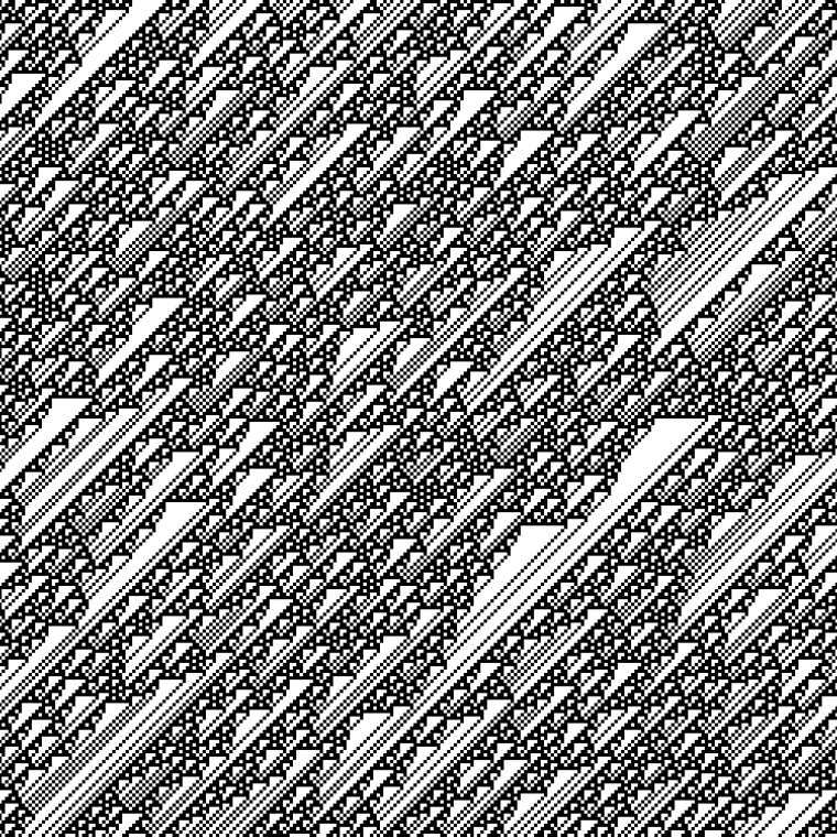
example of rule 73

-
RE: How can I split a path into multiple segments?posted in General Discussion
@jansindl3r keep in mind that in a Bezier curve time and distance do not correlate. if you construct a point at time .1 it will not be at one tenth of the curve length.
afaik the most common technique to get similar distances is to calculate lots of points on the curve(s), calculate some distances and select the closest points.
this link has some very helpful information.
good luck.
-
RE: How to mirror/flip a object?posted in General Discussion
@habakuk nice to read that you can use some of the code!
about the lissajous: I am not sure what exactly you want to achieve. the german wiki entry has vizualisations for a few values. you might want to change the value for
aandband alsodelta, eg:a = 1 b = 3 delta = pi/4I do not have your variable font so I cannot test this but I was wondering why you added the plus and minus 20 here:
curr_axis1 = ip(axis1_min + 20, axis1_max - 20, x)
curr_axis2 = ip(axis2_min + 20, axis2_max - 20, y)
lastly if you want to draw the shadow in the back, just put the lines of code before you call the pink drawing. you might then use the
savedState()so draw it without the mirroring.good luck, jo!
-
RE: A deeper bevel on lineJoin()?posted in General Discussion
and thanks to @gferreira who helped me getting the initial bits!
-
RE: A deeper bevel on lineJoin()?posted in General Discussion
I was working on a fold-font system a few years ago. it took some time to get the trigonometry right. but once that was solved the possibilities were endless ...
so the new alphabet could be rendered with different stroke weights


scaling in the x

or y direction
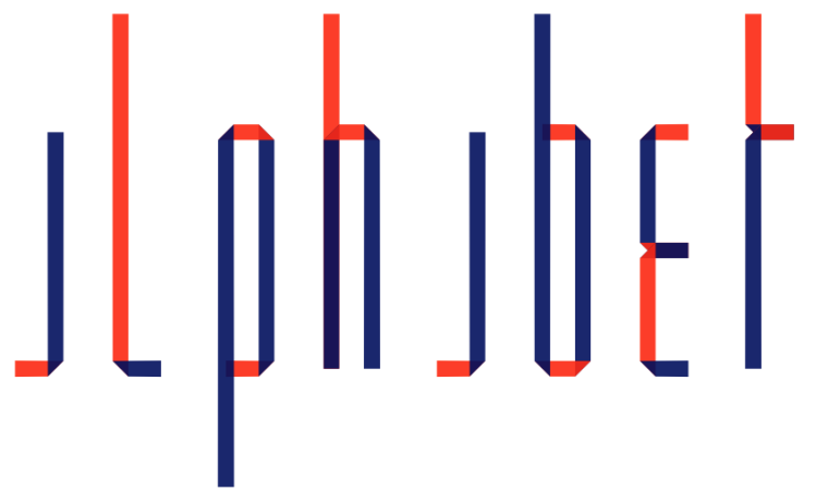
and there could be multi-liners
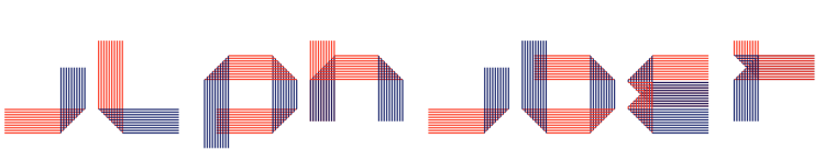
seems like i did not compensate for the stroke weight at the end of a stroke but the system could be used for any collection of xy-points

it is all a bit messy but let me know if you need some bits.
-
RE: Variable portraitposted in Tutorials
hi @eduairet
you can submit a string of characters to the random choice function:chars = 'aeiou' print (random.choice(chars))any call of a ‘drawing function’ will make a new Page. Remove the
translate(0, 2)to not have the blank page.Finally getting the image pixel color takes some time. Try to move stuff outside of the loops if they do not change. Eg try a loop outside the
ranLetters()function to get and store the pixel colors, so you do not have to do that for every page.pix_cols = {} for x in range(0, w, s): for y in range(0, h, s): pix_cols[(x, y)] = imagePixelColor(path, (x, y))then inside the loop just ask for the stored value:
color = pix_cols[(x, y)]also these three lines do not change so they could be outside of the loop:
font("League Spartan Variable")
fontSize(s)
lineHeight(s * 0.75)
good luck!
-
RE: Tutorial request: how to animate a variable fontposted in Tutorials
@hanafolkwang hi, this is half a year too late and probably not even what you were looking for but I made a few more examples to generate .gifs of variable fonts.
Since there are several files I put them on github.
-
RE: Tutorial request: BezierPath() to penposted in Tutorials
thanks @gferreira and @frederik!
great help. i managed to botch my rough attempt at type on a curve.# -------------------------------- # imports from fontTools.pens.basePen import BasePen # -------------------------------- # settings pw = ph = 400 r = 89 angle = pi * 3.1 baseline = ph/2 + r txt = 'HELLO' tang_f = .333 # tangent factor center = pw/2, baseline focus = pw/2, baseline - r # -------------------------------- # functions def ip(a, b, f): return a + (b-a) * f def conv_point(p): x, y = p f = (x - pw/2) / (pw/2) a = -angle/2 * f x_conv = center[0] + cos(a + pi/2) * (r + y - baseline) y_conv = center[1] + sin(a + pi/2) * (r + y - baseline) - r return x_conv, y_conv class convert_path_pen(BasePen): def __init__(self, targetPen): self.targetPen = targetPen def _moveTo(self, pt): self.targetPen.moveTo( conv_point(pt) ) self.prev_pt = pt def _lineTo(self, pt): if self.prev_pt[0] == pt[0]: self.targetPen.lineTo( conv_point(pt) ) else: tang_1 = ip(self.prev_pt[0], pt[0], tang_f), ip(self.prev_pt[1], pt[1], tang_f) tang_2 = ip(self.prev_pt[0], pt[0], 1-tang_f), ip(self.prev_pt[1], pt[1], 1-tang_f) self.targetPen.curveTo(conv_point(tang_1), conv_point(tang_2), conv_point(pt)) self.prev_pt = pt def _curveToOne(self, tang_1, tang_2, pt): self.targetPen.curveTo(conv_point(tang_1), conv_point(tang_2), conv_point(pt)) self.prev_pt = pt def _closePath(self): self.targetPen.closePath() # -------------------------------- # drawings path = BezierPath() path.text(txt, font="Helvetica", fontSize = 80, align = 'center', offset=(0, baseline)) newPage(pw, ph) trans_path = BezierPath() trans_pen = convert_path_pen( trans_path ) path.drawToPen( trans_pen ) drawPath(trans_path)obligatory gifs

-
RE: Animation tutorial screencastposted in Tutorials
@long-season
at what part are you stuck?did you have a look at the documentation?
http://www.drawbot.com/content/text/drawingText.html